“The idea behind digital computers may be explained by saying that
these machines are intended to carry out any operations which could be
done by a human computer.” - Alan Turing
Turing Machines (TMs) are named after (not by) their
inventor, Alan Turing. The TM is certainly the most influential general
model of computation, though not the most practical. It is simple, yet
apparently universal in terms of what can be computed.
In a Turing Machine, the input is written onto an infinite (otherwise
blank) tape. The TM has a read/write head that is initially positioned
at the start of the input string. Computation is controlled by a
deterministic finite automaton: which transition to take depends on
the state of the automaton, and
the tape character under the read/write head;
the transition specifies
a tape character to write (overwriting the character that was just
read),
the new automaton state, and
whether the read/write head should move right by one character or or
left by one character.
The TM repeatedly takes transitions (moving the head and reading and
writing the tape) until it transitions to one of two special automaton
states: if it transitions to the halt-and-accept state then
computation ends and the input is accepted; if it transitions to the
halt-and-reject state then computation ends and the input is
rejected.
This has two important consequences:
The TM can move back and forth over the input, reading it as many
times as it wishes. (Contrast this with DFAs, which see each character
of the input exactly once.)
There is no guarantee that a Turing Machine will ever reach
the halt-and-accept or halt-and-reject states. Unlike a DFA (which will
accept or reject), a TM has three possible outcomes: accept, reject, or
never produce an answer.
Psychological Motivation
Other models of general computation (including lambda calculus, which
later became the core of modern functional programming languages) were
proposed before Turing Machines. But TMs were particularly influential,
perhaps because Turing’s original 1936 paper, On Computable Numbers,
with an application to the Estschedungsproblem [i.e., Decision
Problem] , directly modeled Turing Machines on the capabilities of
a human doing calculations, e.g.,
Humans do calculations on paper; using a long one-dimensional strip
of paper instead of a normal page would be less convienient, but it
wouldn’t change what calculations could be performed;
Dividing the strip of paper into squares and writing one character
per square wouldn’t change what the human could calculate.
There are only finitely many different symbols that could be written
in any particular square. (Even at some insane resolution like 1 million
dots per inch, a printer can only print a large but finite number of
different images in any particular square. Coming up with infinitely
many different symbols to draw in a finite square on the paper requires
arbitrarily string magnifying glasses to distinguish different
symbols.)
At any given instant, there’s a bound on how many squares on the
paper the human can observe; to see more squares, the human would have
to move their head or eyes and make successive observations.
There are only finitely many things the human could be thinking at
any given instant; Turing calls these “states of mind” and argues that
the number of such states is finite because the brain is finite and (as
with symbols on paper) if the number of possibilities were infinite then
the difference between different states of mind would be infinitely
small. This is perhaps the least convincing of Turing’s arguments, but
it’s not obviously wrong.
These assumptions about humans then translated into the infinite
tape, finite controller, etc., of a Turing Machine. Consequently, it’s
plausible that a Turing Machines can calculate anything a human could,
and hence TMs serve as a “universal” model of computation.
In contrast, previous proposals for general models of computation
could be shown to calculate everything one could think of, yet there was
always the worry that one might eventually find other reasonable
calculations that a human could do but were impossible in the model.
An Example
For Turing Machines with a small number of automaton states and
transitions, we can define the TM by drawing a diagram. As with DFAs and
NFAs, the graph shows the states and the transitions. The label \(a\to b, D\) means “we take this transition
if the current tape symbol is \(a\); if
we take this transition, overwrite the \(a\) on the tape with \(b\), and move one step in direction \(D\) on the tape (right or left).”
Example
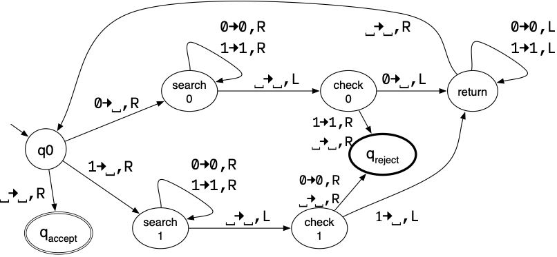
The following Turing Machine checks whether its input is a palindrome
of even length: It works roughly as follows: > >-
In the start state “q0” the TM checks the first symbol of the input.
>- If it’s 1, we erase it and move right. The TM then moves to the
last symbol of the input (by moving right without modifying the tape
until it finds the blank symbol following the input, and then moving one
step left). It then checks whether that last symbol is 1. > > If
not, the TM halts and rejects. > > If so, the TM erases that last
1 (leaving what is hopefully a shorter palindrome on the tape). It also
switches to the “return” state, which moves the TM left to the first
remaining symbol (by moving left until it sees the blank before the
first symbol, and taking one step right). Then the TM restarts and
checks that the remaining characters also form a palindrome. > >-
If the first character was a 0, the TM takes the upper path, which
performs similar steps (erase the leading 0, move to the last symbol,
confirm it’s 0, erase the trailing 0, and then move back to the start of
the remaining string). >- If the first character is a blank, it means
that the input is (or has become) and empty string; this is definitely
an even-length palindrome, and so the TM halts and accepts.
Turing Machine Variations
For DFAs, we argued that adding other capabilities such as
nondeterminism or spontaneous \(\epsilon\)-transitions didn’t change what
can be computed.
For Turing Machines, many other extensions have been investigated,
and all have turned out to be equivalent to the original TM. For
example, we could add any or all of the following extensions, and any
calculations the extended TM could perform could be simulated by an
ordinary basic TM as defined above:
Adding the option to write or not on each step;
Adding the option to stay-in-place rather than moving left or
right;
Adding any finite number of finite “registers” (variables with
finite storage capacity);
Allowing transitions to erase the entire tape in one step;
Allowing multiple tapes, each with independent read/write
heads;
Allowing the read/write head to read \(B\) symbols at the head (instead of just
one);
Making the tape two-dimensional (with a head that can move
up/down/left/right);
Making the controlling automaton an NFA instead of a DFA;
and many other variations.
The Church-Turing Thesis
Definition
The Church-Turing Thesis (also known as Church’s
Thesis or Turing’s Thesis) says that any realistic model
of general computation will be equivalent in power to Turing Machines.
> It’s called a “thesis” rather than a “theorem” because it’s
impossible to prove unless we can formally define what counts as a
realistic model of computation, which seems difficult. > Empirically,
however, it seems true. Many other models of computation have
been proposed, and they all have turned out to be equivalent to Turing
Machines (or in rare cases, less powerful than Turing Machines).
Universal Turing Machines
We have already seen examples of theoretical machines that can
simulate other machines. For example, we can use DFAs to simulate NFAs
(subset construction), and we can use one DFA to simulate two DFAs
running in parallel (product automaton).
Similarly, one Turing Machine can simulate another. In fact, there
are so-called Universal Turing Machines (UTMs) that can
simulate any Turing Machine we’d like; when we start the UTM, the tape
contains an encoding of the machine to simulate and an encoding of the
input to feed to the simulated machine. Then the UTM accepts, rejects,
or runs forever depending on what that machine would do on that
input.
This is convenient, because we don’t have to imagine building a new
TM for every different problem (the way we would build a different DFA
every time we want to check strings against a different regular
expression). Instead, we could have a single UTM, and tell it (on the
tape) which TM we want to emulate and what input it should use.
We know that Universal Turing Machines exist because specific
examples have been constructed. The first UTM was proposed by Alan
Turing in his original paper. A number of other TMs have been proved
universal since then, with the simplest having only 2 automaton states
and 3 non-blank tape symbols (Smith and Wolfram, 2007).
Variations on UTMs also let us simulate any given TM on any given
input for a specific number of steps, or until something interesting
happens on the (simulated) tape. We could also simulate two TMs running
at once (by multitasking; taking one step on one simulated TM, and then
One step on a second simulated TM, then back to the first, and so
on).
The upshot: When thinking how a Turing Machine might
solve a problem (designing the algorithm), we are free to say that at
some point the TM can start simulating some other machine on some other
input, and watch what happens.
 It works roughly as follows: > >-
In the start state “q0” the TM checks the first symbol of the input.
>- If it’s 1, we erase it and move right. The TM then moves to the
last symbol of the input (by moving right without modifying the tape
until it finds the blank symbol following the input, and then moving one
step left). It then checks whether that last symbol is 1. > > If
not, the TM halts and rejects. > > If so, the TM erases that last
1 (leaving what is hopefully a shorter palindrome on the tape). It also
switches to the “return” state, which moves the TM left to the first
remaining symbol (by moving left until it sees the blank before the
first symbol, and taking one step right). Then the TM restarts and
checks that the remaining characters also form a palindrome. > >-
If the first character was a 0, the TM takes the upper path, which
performs similar steps (erase the leading 0, move to the last symbol,
confirm it’s 0, erase the trailing 0, and then move back to the start of
the remaining string). >- If the first character is a blank, it means
that the input is (or has become) and empty string; this is definitely
an even-length palindrome, and so the TM halts and accepts.
It works roughly as follows: > >-
In the start state “q0” the TM checks the first symbol of the input.
>- If it’s 1, we erase it and move right. The TM then moves to the
last symbol of the input (by moving right without modifying the tape
until it finds the blank symbol following the input, and then moving one
step left). It then checks whether that last symbol is 1. > > If
not, the TM halts and rejects. > > If so, the TM erases that last
1 (leaving what is hopefully a shorter palindrome on the tape). It also
switches to the “return” state, which moves the TM left to the first
remaining symbol (by moving left until it sees the blank before the
first symbol, and taking one step right). Then the TM restarts and
checks that the remaining characters also form a palindrome. > >-
If the first character was a 0, the TM takes the upper path, which
performs similar steps (erase the leading 0, move to the last symbol,
confirm it’s 0, erase the trailing 0, and then move back to the start of
the remaining string). >- If the first character is a blank, it means
that the input is (or has become) and empty string; this is definitely
an even-length palindrome, and so the TM halts and accepts.